图像处理
目录
图像处理
欢迎阅读 dask-image 快速入门指南。
设置你的环境
安装额外依赖项
我们首先安装 scikit-image 库,以便更轻松地访问其中的示例图像数据。
如果你在自己的计算机上运行此 notebook 而不是在 mybinder 环境中运行,则还需要确保你的 Python 环境包含: * dask * dask-image * python-graphviz * scikit-image * matplotlib * numpy
你可以参考 dask-examples 仓库使用的完整依赖项列表,该列表在 `binder/environment.yml 文件中提供 <https://github.com/dask/dask-examples/blob/main/binder/environment.yml>`__(请注意,nomkl 包不适用于 Windows 用户): https://github.com/dask/dask-examples/blob/main/binder/environment.yml
导入 dask-image
当你导入 dask-image 时,请务必在两个单词之间使用下划线而不是连字符。
[1]:
import dask_image.imread
import dask_image.ndfilters
import dask_image.ndmeasure
import dask.array as da
我们还将使用 matplotlib 在此 notebook 中显示图像结果。
[2]:
import matplotlib.pyplot as plt
%matplotlib inline
获取示例数据
在本教程中,我们将使用来自 scikit-image 库的一些示例图像数据。这些图像非常小,但能让我们演示 dask-image 的功能。
让我们下载并保存宇航员 Eileen Collins 的一张公共领域图像到临时目录。此图像最初从 NASA Great Images 数据库 https://flic.kr/p/r9qvLn 下载,但我们将使用 scikit-image 的 data.astronaut() 方法访问它。
[3]:
!mkdir temp
[4]:
import os
from skimage import data, io

output_filename = os.path.join('temp', 'astronaut.png')
io.imsave(output_filename, data.astronaut())
超大型数据集通常无法将所有数据放入单个文件中,因此我们将此图像切成四部分,并将图像块保存到第二个临时目录中。这将让你更好地了解如何在真实数据集上使用 dask-image。
[5]:
!mkdir temp-tiles
[6]:
io.imsave(os.path.join('temp-tiles', 'image-00.png'), data.astronaut()[:256, :256, :])  # top left
io.imsave(os.path.join('temp-tiles', 'image-01.png'), data.astronaut()[:256, 256:, :])  # top right
io.imsave(os.path.join('temp-tiles', 'image-10.png'), data.astronaut()[256:, :256, :])  # bottom left
io.imsave(os.path.join('temp-tiles', 'image-11.png'), data.astronaut()[256:, 256:, :])  # bottom right
现在我们已经保存了一些数据,让我们练习使用 dask-image 读取文件并处理图像。
读取图像数据
读取单个图像
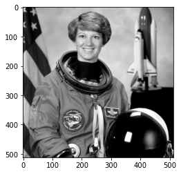
让我们使用 dask-image imread() 加载宇航员 Eileen Collins 的公共领域图像。此图像最初从 NASA Great Images 数据库 https://flic.kr/p/r9qvLn 下载。
[7]:
import os
filename = os.path.join('temp', 'astronaut.png')
print(filename)
temp/astronaut.png
[8]:
astronaut = dask_image.imread.imread(filename)
print(astronaut)
plt.imshow(astronaut[0, ...])  # display the first (and only) frame of the image
dask.array<_map_read_frame, shape=(1, 512, 512, 3), dtype=uint8, chunksize=(1, 512, 512, 3), chunktype=numpy.ndarray>
[8]:
<matplotlib.image.AxesImage at 0x7f0fb95fff40>
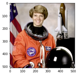
这创建了一个形状为 shape=(1, 512, 512, 3) 的 dask 数组。这意味着它包含一帧图像,具有 512 行、512 列和 3 个颜色通道。
由于图像相对较小,它完全适合一个 dask-image chunk 中,其 chunksize=(1, 512, 512, 3)。
读取多个图像
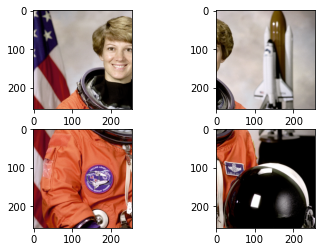
在许多情况下,你的磁盘上可能存储着多个图像,例如:image_00.png, image_01.png, … image_NN.png。这些可以作为多个图像帧读入 dask 数组。
这里我们将宇航员图像分割成四个不重叠的块: * image_00.png = 左上角图像 (索引 0,0) * image_01.png = 右上角图像 (索引 0,1) * image_10.png = 左下角图像 (索引 1,0) * image_11.png = 右下角图像 (索引 1,1)
这个文件名模式可以使用 regex 匹配:image-*.png
[9]:
!ls temp-tiles
image-00.png image-01.png image-10.png image-11.png
[10]:
import os
filename_pattern = os.path.join('temp-tiles', 'image-*.png')
tiled_astronaut_images = dask_image.imread.imread(filename_pattern)
print(tiled_astronaut_images)
dask.array<_map_read_frame, shape=(4, 256, 256, 3), dtype=uint8, chunksize=(1, 256, 256, 3), chunktype=numpy.ndarray>
这创建了一个形状为 shape=(4, 256, 256, 3) 的 dask 数组。这意味着它包含四帧图像;每帧有 256 行、256 列和 3 个颜色通道。
在这个特定情况下有四个 chunk。这里的每个图像帧都是一个单独的 chunk,其 chunksize=(1, 256, 256, 3)。
[11]:
fig, ax = plt.subplots(nrows=2, ncols=2)
ax[0,0].imshow(tiled_astronaut_images[0])
ax[0,1].imshow(tiled_astronaut_images[1])
ax[1,0].imshow(tiled_astronaut_images[2])
ax[1,1].imshow(tiled_astronaut_images[3])
plt.show()
对图像应用你自己的自定义函数
接下来你会想进行一些图像处理,并对图像应用一个函数。
我们将使用一个非常简单的例子:将 RGB 图像转换为灰度图像。但你也可以使用此方法对 dask 图像应用任意函数。要将我们的图像转换为灰度图像,我们将使用以下方程计算亮度(参考 pdf)
Y = 0.2125 R + 0.7154 G + 0.0721 B
我们将按照如下方式编写此方程的函数
[12]:
def grayscale(rgb):
    result = ((rgb[..., 0] * 0.2125) +
              (rgb[..., 1] * 0.7154) +
              (rgb[..., 2] * 0.0721))
    return result
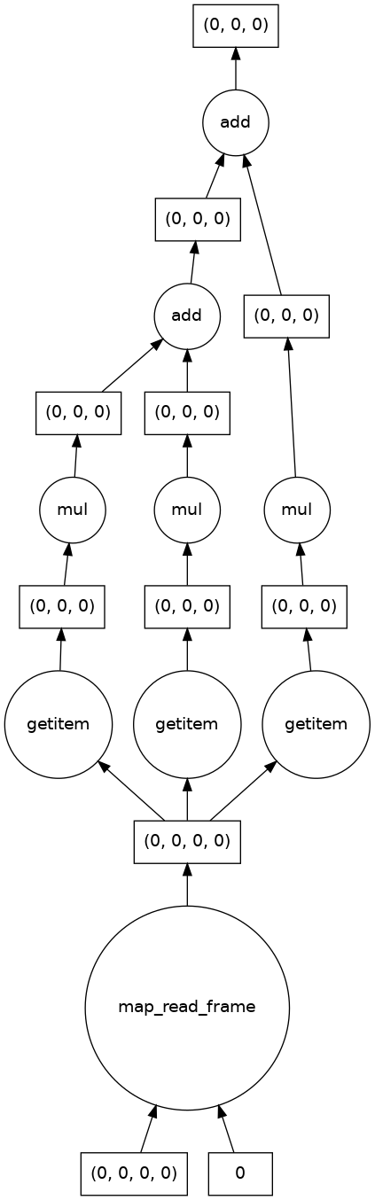
让我们将此函数应用于我们以单个文件形式读入的宇航员图像,并可视化计算图。
(可视化计算图通常不是必需的,但了解 dask 在幕后做什么很有帮助,而且它对于调试问题也非常有用。)
[13]:
single_image_result = grayscale(astronaut)
print(single_image_result)
single_image_result.visualize()
dask.array<add, shape=(1, 512, 512), dtype=float64, chunksize=(1, 512, 512), chunktype=numpy.ndarray>
[13]:
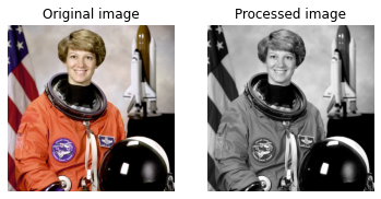
我们还看到结果的形状中不再有三个颜色通道,并且输出图像符合预期。
[14]:
print("Original image dimensions: ", astronaut.shape)
print("Processed image dimensions:", single_image_result.shape)

fig, (ax0, ax1) = plt.subplots(nrows=1, ncols=2)
ax0.imshow(astronaut[0, ...])            # display the first (and only) frame of the image
ax1.imshow(single_image_result[0, ...], cmap='gray')  # display the first (and only) frame of the image

# Subplot headings
ax0.set_title('Original image')
ax1.set_title('Processed image')

# Don't display axes
ax0.axis('off')
ax1.axis('off')

# Display images
plt.show(fig)
Original image dimensions:  (1, 512, 512, 3)
Processed image dimensions: (1, 512, 512)
易并行问题
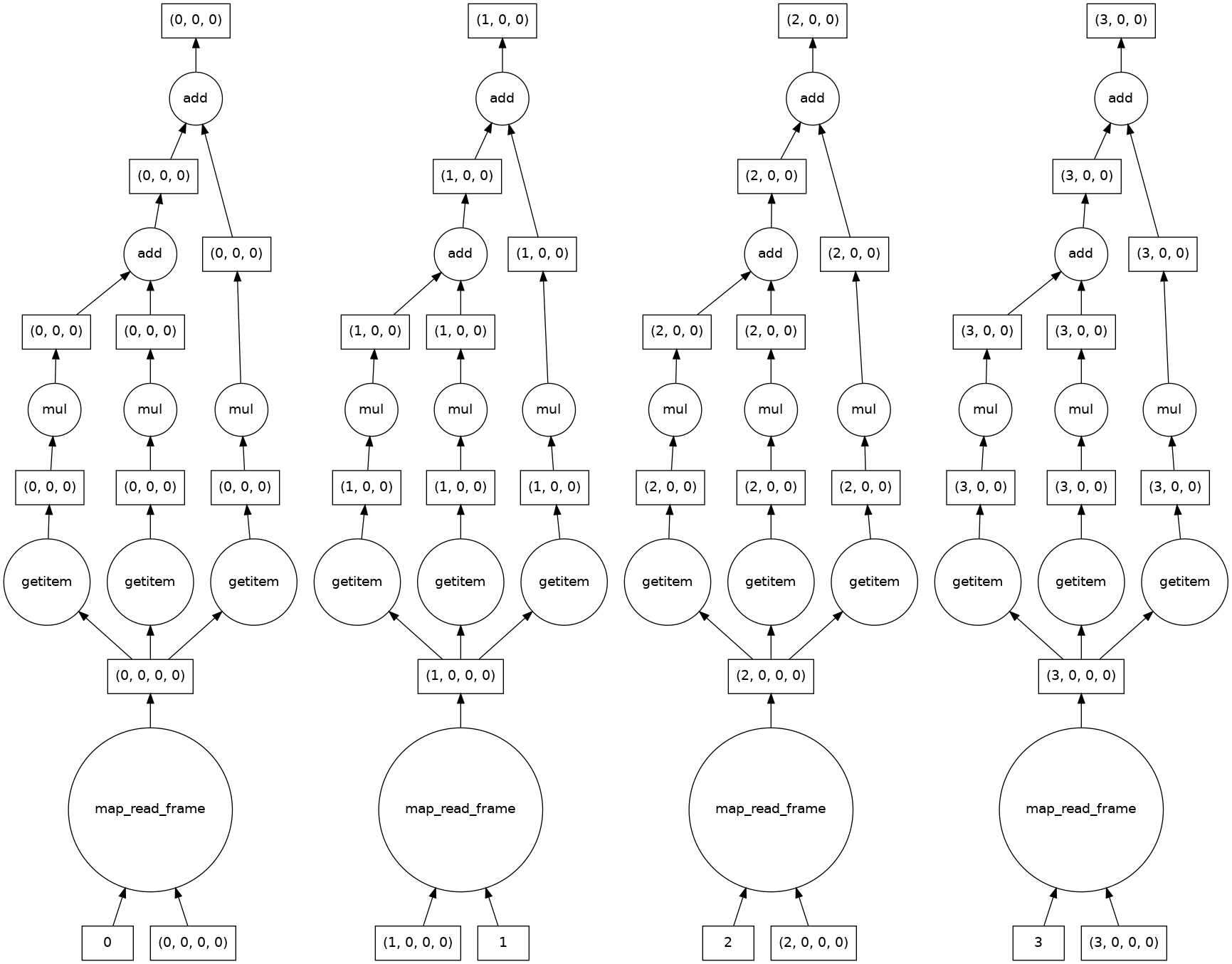
将函数应用于多个图像或 dask chunk 的语法是相同的。这是一个易并行问题的例子,我们看到 dask 会自动为每个 chunk 创建一个计算图。
[15]:
result = grayscale(tiled_astronaut_images)
print(result)
result.visualize()
dask.array<add, shape=(4, 256, 256), dtype=float64, chunksize=(1, 256, 256), chunktype=numpy.ndarray>
[15]:
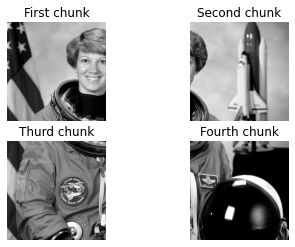
让我们看一下结果。
[16]:
fig, ((ax0, ax1), (ax2, ax3)) = plt.subplots(nrows=2, ncols=2)
ax0.imshow(result[0, ...], cmap='gray')
ax1.imshow(result[1, ...], cmap='gray')
ax2.imshow(result[2, ...], cmap='gray')
ax3.imshow(result[3, ...], cmap='gray')

# Subplot headings
ax0.set_title('First chunk')
ax1.set_title('Second chunk')
ax2.set_title('Thurd chunk')
ax3.set_title('Fourth chunk')

# Don't display axes
ax0.axis('off')
ax1.axis('off')
ax2.axis('off')
ax3.axis('off')

# Display images
plt.show(fig)
合并部分图像
好的,看起来相当不错!但是我们如何将这些图像块合并起来呢?
到目前为止,我们进行计算时不需要任何来自相邻像素的信息。但是有很多函数(例如 dask-image ndfilters 中的函数)确实需要这些信息来获得准确的结果。如果你不告诉 dask 如何合并图像,可能会产生不想要的边缘效应。
Dask 有几种合并 chunk 的方法:Stack, Concatenate, and Block。
Block 非常通用,所以我们将在下一个例子中使用它。你只需传入一个列表(或列表的列表)来告诉 dask 图像 chunk 之间的空间关系。
[17]:
data = [[result[0, ...], result[1, ...]],
        [result[2, ...], result[3, ...]]]
combined_image = da.block(data)
print(combined_image.shape)
plt.imshow(combined_image, cmap='gray')
(512, 512)
[17]:
<matplotlib.image.AxesImage at 0x7f0fb8187e80>
分割分析管道
我们将通过一个简单的图像分割和分析管道,包含三个步骤: 1. 过滤 1. 分割 1. 分析
过滤
大多数分析管道需要一定程度的图像预处理。dask-image 通过 dask-image ndfilters 提供多种内置滤波器。
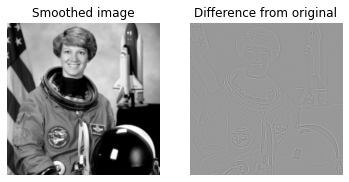
通常可以使用高斯滤波器在分割前平滑图像。这会导致图像损失一些清晰度,但可以提高依赖图像阈值处理的方法的分割质量。
[18]:
smoothed_image = dask_image.ndfilters.gaussian_filter(combined_image, sigma=[1, 1])
我们看到平滑后的图像有轻微的模糊。
[19]:
fig, (ax0, ax1) = plt.subplots(nrows=1, ncols=2)
ax0.imshow(smoothed_image, cmap='gray')
ax1.imshow(smoothed_image - combined_image, cmap='gray')

# Subplot headings
ax0.set_title('Smoothed image')
ax1.set_title('Difference from original')

# Don't display axes
ax0.axis('off')
ax1.axis('off')

# Display images
plt.show(fig)
由于高斯滤波器使用相邻像素的信息,计算图看起来比我们之前看到的要复杂。这不再是易并行的。在可能的情况下,dask 会将四个图像 chunk 的计算分开处理,但在边缘附近必须结合不同 chunk 的信息。
[20]:
smoothed_image.visualize()
[20]:
分割
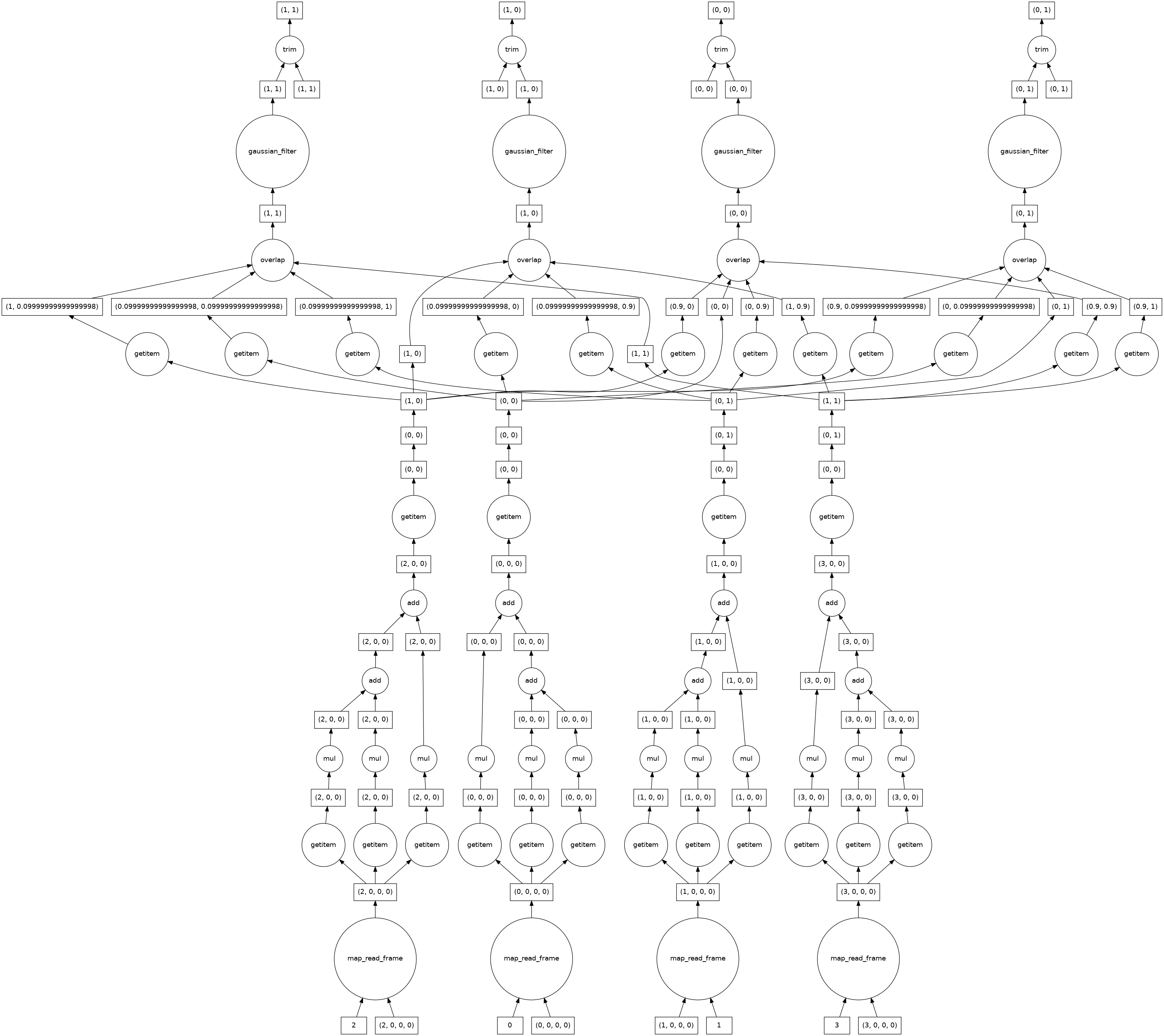
图像预处理后,我们从数据中分割出感兴趣区域。我们将使用一个简单的任意阈值作为截止值,即平滑图像最大强度的 75%。
[21]:
threshold_value = 0.75 * da.max(smoothed_image).compute()
print(threshold_value)
190.5550614819934
[22]:
threshold_image = smoothed_image > threshold_value
plt.imshow(threshold_image, cmap='gray')
[22]:
<matplotlib.image.AxesImage at 0x7f0fb82f9d00>
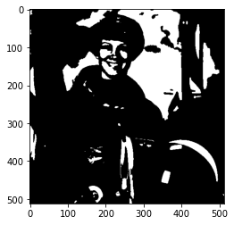
接下来,我们标记阈值以上每个连接像素区域。为此,我们使用 dask-image ndmeasure 中的 label 函数。这将返回标签图像和标签数量。
[23]:
label_image, num_labels = dask_image.ndmeasure.label(threshold_image)
[24]:
print("Number of labels:", int(num_labels))
plt.imshow(label_image, cmap='viridis')
Number of labels: 78
[24]:
<matplotlib.image.AxesImage at 0x7f0fb801c760>
分析
dask-image ndmeasure 中有许多内置函数可用于定量分析。
我们将使用 dask_image.ndmeasure.mean() 和 dask_image.ndmeasure.standard_deviation() 函数,并使用 dask_image.ndmeasure.labeled_comprehension() 将它们应用于每个标签区域。
[25]:
index = list(range(int(num_labels)))  # Note that we're including the background label=0 here, too.
out_dtype = float  # The data type we want to use for our results.
default = None     # The value to return if an element of index does not exist in the label image.
mean_values = dask_image.ndmeasure.labeled_comprehension(combined_image, label_image, index, dask_image.ndmeasure.mean, out_dtype, default, pass_positions=False)
print(mean_values.compute())
[ 90.87492186 194.69185981 207.76964212 215.16959146 196.92609412
 206.50032105 217.0948     211.0477766  205.68146    208.61031956
 212.43803803 201.39967857 210.291275   198.3529809  201.21037636
 214.13041176 200.9344975  201.85547778 194.46485714 202.60302231
 205.20927983 203.72510602 205.94798756 205.88514047 207.33728
 216.13305227 206.7058     211.6957     211.75921279 224.71301613
 249.08085    215.87763779 198.27655577 213.67658483 205.65810758
 197.46586082 202.35786579 199.16034783 216.27194848 200.69137594
 220.99142573 207.66165    234.37771667 224.00188182 229.2705
 232.9163     187.1873     236.16183793 223.7469     187.813475
 227.4778     244.17155    225.49225806 239.4951     218.7795
 242.99015132 232.4975218  201.98308947 230.57158889 212.82135217
 242.21528571 241.32428889 228.722932   220.1454     239.55
 246.5        241.53348    236.28736    244.84466624 242.09528
 203.37236667 209.34061875 213.76621346 247.53468249 252.488826
 208.5659     197.72356    203.13211   ]
由于我们在索引中包含了标签 0,所以第一个平均值比其他值低很多并不奇怪——它是分割截止阈值以下的背景区域。
让我们也计算灰度图像中像素值的标准差。
[26]:
stdev_values = dask_image.ndmeasure.labeled_comprehension(combined_image, label_image, index, dask_image.ndmeasure.standard_deviation, out_dtype, default, pass_positions=False)
最后,让我们将分析结果加载到 pandas 表中,然后将其保存为 csv 文件。
[27]:
import pandas as pd

df = pd.DataFrame()
df['label'] = index
df['mean'] = mean_values.compute()
df['standard_deviation'] = stdev_values.compute()

df.head()
[27]:
| 标签 | 平均值 | 标准差 | |
|---|---|---|---|
| 0 | 0 | 90.874922 | 65.452828 |
| 1 | 1 | 194.691860 | 2.921235 |
| 2 | 2 | 207.769642 | 11.411058 |
| 3 | 3 | 215.169591 | 9.193374 |
| 4 | 4 | 196.926094 | 5.215053 |
[28]:
df.to_csv('example_analysis_results.csv')
print('Saved example_analysis_results.csv')
Saved example_analysis_results.csv
下一步
希望本指南能帮助你开始使用 dask-image。
文档
你可以在 dask-image 文档 和 API 参考 中阅读更多关于 dask-image 的内容。dask 的文档在这里。
dask-examples 仓库包含许多其他示例 notebook: https://github.com/dask/dask-examples
使用 dask distributed 进行扩展
如果你想将 dask 任务发送到计算集群进行分布式处理,你应该查看 dask distributed。还有一个可用的 快速入门指南。
使用 zarr 保存图像数据
在某些情况下,图像处理后可能需要保存大量数据,zarr 是一个你可能会觉得有用的 python 库。