使用 Dask 进行超参数优化
目录
实时 Notebook
您可以在 实时会话 中运行此 Notebook ![]() ,或在 Github 上查看。
,或在 Github 上查看。
使用 Dask 进行超参数优化
每个机器学习模型在训练开始前都会指定一些值。这些值有助于使模型适应数据,但必须在看到任何训练数据之前给出。例如,在 Scikit-learn 的 LogisiticRegression 中,这可能是 penalty 或 C。这些在任何训练数据之前出现的值被称为“超参数”。典型用法如下所示:
from sklearn.linear_model import LogisiticRegression
from sklearn.datasets import make_classification

X, y = make_classification()
est = LogisiticRegression(C=10, penalty="l2")
est.fit(X, y)
这些超参数会影响预测的质量。例如,如果在上面的示例中 C 太小,估计器的输出将无法很好地拟合数据。
确定这些超参数的值很困难。事实上,Scikit-learn 有一整个文档页面专门介绍如何找到最佳值:https://scikit-learn.cn/stable/modules/grid_search.html
Dask 为超参数优化提供了一些新技术和机会。其中一个机会涉及提前停止训练以限制计算。自然地,这需要某种方式来停止和重新开始训练(在 Scikit-learn 术语中称为 partial_fit 或 warm_start)。
当搜索复杂且有许多搜索参数时,这尤其有用。很好的例子是大多数深度学习模型,它们有专门处理大量数据的算法,但在提供基本超参数(例如,“学习率”、“动量”或“权重衰减”)方面存在困难。
本 Notebook 将介绍
设置一个实际示例
如何使用
HyperbandSearchCV,包括理解
HyperbandSearchCV的输入参数运行超参数优化
如何从
HyperbandSearchCV访问信息
本 Notebook 特别不会展示促使使用 HyperbandSearchCV 的性能比较。HyperbandSearchCV 以最少的训练找到高分;但是,这是一个关于如何使用它的教程。所有性能比较都放在了解更多 部分。
[1]:
%matplotlib inline
设置 Dask
[2]:
from distributed import Client
client = Client(processes=False, threads_per_worker=4,
                n_workers=1, memory_limit='2GB')
client
[2]:
客户端
客户端-6ab1bd16-0de1-11ed-a383-000d3a8f7959
| 连接方法: Cluster 对象 | 集群类型: distributed.LocalCluster |
| 仪表板: http://10.1.1.64:8787/status |
集群信息
LocalCluster
3d7b2964
| 仪表板: http://10.1.1.64:8787/status | 工作节点 1 |
| 总线程数 4 | 总内存: 1.86 GiB |
| 状态: 运行中 | 使用进程: 否 |
调度器信息
调度器
调度器-c1bf35f0-8caf-4476-9919-060006f58f79
| 通信: inproc://10.1.1.64/9091/1 | 工作节点 1 |
| 仪表板: http://10.1.1.64:8787/status | 总线程数 4 |
| 启动时间: 刚刚 | 总内存: 1.86 GiB |
工作节点
工作节点:0
| 通信: inproc://10.1.1.64/9091/4 | 总线程数 4 |
| 仪表板: http://10.1.1.64:37053/status | 内存: 1.86 GiB |
| Nanny: 无 | |
| 本地目录: /home/runner/work/dask-examples/dask-examples/machine-learning/dask-worker-space/worker-uj3a5b08 | |
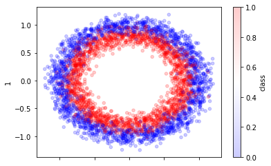
创建数据
[3]:
from sklearn.datasets import make_circles
import numpy as np
import pandas as pd

X, y = make_circles(n_samples=30_000, random_state=0, noise=0.09)

pd.DataFrame({0: X[:, 0], 1: X[:, 1], "class": y}).sample(4_000).plot.scatter(
    x=0, y=1, alpha=0.2, c="class", cmap="bwr"
);
添加随机维度
[4]:
from sklearn.utils import check_random_state

rng = check_random_state(42)
random_feats = rng.uniform(-1, 1, size=(X.shape[0], 4))
X = np.hstack((X, random_feats))
X.shape
[4]:
(30000, 6)
分割和缩放数据
[5]:
from sklearn.model_selection import train_test_split
X_train, X_test, y_train, y_test = train_test_split(X, y, test_size=5_000, random_state=42)
[6]:
from sklearn.preprocessing import StandardScaler
from sklearn.model_selection import train_test_split
scaler = StandardScaler().fit(X_train)

X_train = scaler.transform(X_train)
X_test = scaler.transform(X_test)
[7]:
from dask.utils import format_bytes

for name, X in [("train", X_train), ("test", X_test)]:
    print("dataset =", name)
    print("shape =", X.shape)
    print("bytes =", format_bytes(X.nbytes))
    print("-" * 20)
dataset = train
shape = (25000, 6)
bytes = 1.14 MiB
--------------------
dataset = test
shape = (5000, 6)
bytes = 234.38 kiB
--------------------
现在我们有了训练集和测试集。
创建模型和搜索空间
为了方便起见,让我们使用 Scikit-learn 的 MLPClassifier 作为我们的模型。让我们使用这个有 24 个神经元的模型,并调整一些其他基本超参数。
[8]:
import numpy as np
from sklearn.neural_network import MLPClassifier

model = MLPClassifier()
也可以使用深度学习库。特别是,PyTorch 的 Scikit-Learn 封装 Skorch 与 HyperbandSearchCV 配合良好。
[9]:
params = {
    "hidden_layer_sizes": [
        (24, ),
        (12, 12),
        (6, 6, 6, 6),
        (4, 4, 4, 4, 4, 4),
        (12, 6, 3, 3),
    ],
    "activation": ["relu", "logistic", "tanh"],
    "alpha": np.logspace(-6, -3, num=1000),  # cnts
    "batch_size": [16, 32, 64, 128, 256, 512],
}
超参数优化
HyperbandSearchCV 是 Dask-ML 用来寻找最佳超参数的元估计器。它可以用作 RandomizedSearchCV 的替代方案,通过不将时间浪费在没有前景的超参数上,从而在更短的时间内找到相似的超参数。具体来说,它几乎可以保证以最少的训练找到高性能的模型。
本节将重点介绍
理解
HyperbandSearchCV的输入参数使用
HyperbandSearchCV寻找最佳超参数查看
HyperbandSearchCV的其他用例
[10]:
from dask_ml.model_selection import HyperbandSearchCV
确定输入参数
确定 HyperbandSearchCV 输入参数的一个经验法则是需要知道
训练时间最长的模型将看到的示例数量
要评估的超参数数量
让我们写下本例中这些值应该是什么
[11]:
# For quick response
n_examples = 4 * len(X_train)
n_params = 8

# In practice, HyperbandSearchCV is most useful for longer searches
# n_examples = 15 * len(X_train)
# n_params = 15
在此,训练时间最长的模型将看到 n_examples 个示例。这是所需的数据量,通常由问题难度设定。简单的问题可能只需要通过数据集 10 次;更复杂的问题可能需要通过数据集 100 次。
将采样 n_params 个参数,因此将评估 n_params 个模型。得分较低的模型在看到 n_examples 个示例之前将被终止。这有助于节省计算。
我们如何使用这些值来确定 HyperbandSearchCV 的输入?
[12]:
max_iter = n_params  # number of times partial_fit will be called
chunks = n_examples // n_params  # number of examples each call sees

max_iter, chunks
[12]:
(8, 12500)
这意味着训练时间最长的估计器将看到大约 n_examples 个示例(具体来说是 n_params * (n_examples // n_params))。
应用输入参数
让我们创建一个具有此块大小的 Dask 数组
[13]:
import dask.array as da
X_train2 = da.from_array(X_train, chunks=chunks)
y_train2 = da.from_array(y_train, chunks=chunks)
X_train2
[13]:
|
每次 partial_fit 调用将接收一个块。
这意味着每个块中的示例数量应该(大约)相同,并且应该选择 n_examples 和 n_params 来实现这一点。(例如,对于 100 个示例,应争取 (33, 33, 34) 个示例的块,而不是 (48, 48, 4) 个示例)。
现在让我们使用 max_iter 来创建我们的 HyperbandSearchCV 对象
[14]:
search = HyperbandSearchCV(
    model,
    params,
    max_iter=max_iter,
    patience=True,
)
将执行多少计算?
从 max_iter 和 chunks 不清楚如何确定执行了多少计算。幸运的是,HyperbandSearchCV 有一个 metadata 属性可以预先确定这一点
[15]:
search.metadata["partial_fit_calls"]
[15]:
26
这显示了计算中将执行多少次 partial_fit 调用。metadata 还包括有关创建的模型数量的信息。
到目前为止,所做的只是为计算(以及查看将执行多少计算)做好搜索准备。到目前为止,所有的计算都快速且容易。
执行计算
现在,让我们进行模型选择搜索并找到最佳超参数。这是本 Notebook 的真正核心。此计算将在 Dask 可用的所有硬件上进行。
[16]:
%%time
search.fit(X_train2, y_train2, classes=[0, 1, 2, 3])
/usr/share/miniconda3/envs/dask-examples/lib/python3.9/site-packages/dask_ml/model_selection/_incremental.py:641: VisibleDeprecationWarning: Creating an ndarray from ragged nested sequences (which is a list-or-tuple of lists-or-tuples-or ndarrays with different lengths or shapes) is deprecated. If you meant to do this, you must specify 'dtype=object' when creating the ndarray.
  cv_results = {k: np.array(v) for k, v in cv_results.items()}
/usr/share/miniconda3/envs/dask-examples/lib/python3.9/site-packages/dask_ml/model_selection/_hyperband.py:455: VisibleDeprecationWarning: Creating an ndarray from ragged nested sequences (which is a list-or-tuple of lists-or-tuples-or ndarrays with different lengths or shapes) is deprecated. If you meant to do this, you must specify 'dtype=object' when creating the ndarray.
  cv_results = {k: np.array(v) for k, v in cv_results.items()}
CPU times: user 3.54 s, sys: 661 ms, total: 4.2 s
Wall time: 3.42 s
[16]:
HyperbandSearchCV(estimator=MLPClassifier(), max_iter=8,
                  parameters={'activation': ['relu', 'logistic', 'tanh'],
                              'alpha': array([1.00000000e-06, 1.00693863e-06, 1.01392541e-06, 1.02096066e-06,
       1.02804473e-06, 1.03517796e-06, 1.04236067e-06, 1.04959323e-06,
       1.05687597e-06, 1.06420924e-06, 1.07159340e-06, 1.07902879e-06,
       1.08651577e-06, 1.09405471e-06, 1.10164595e-06, 1.1...
       9.01477631e-04, 9.07732653e-04, 9.14031075e-04, 9.20373200e-04,
       9.26759330e-04, 9.33189772e-04, 9.39664831e-04, 9.46184819e-04,
       9.52750047e-04, 9.59360829e-04, 9.66017480e-04, 9.72720319e-04,
       9.79469667e-04, 9.86265846e-04, 9.93109181e-04, 1.00000000e-03]),
                              'batch_size': [16, 32, 64, 128, 256, 512],
                              'hidden_layer_sizes': [(24,), (12, 12),
                                                     (6, 6, 6, 6),
                                                     (4, 4, 4, 4, 4, 4),
                                                     (12, 6, 3, 3)]},
                  patience=True)
仪表板在此运行时将处于活动状态。它将显示哪些工作节点正在运行 partial_fit 和 score 调用。这大约需要 10 秒。
集成
HyperbandSearchCV 遵循 Scikit-learn API,并模仿 Scikit-learn 的 RandomizedSearchCV。这意味着它“开箱即用”。所有 Scikit-learn 属性和方法都可用
[17]:
search.best_score_
[17]:
0.8122
[18]:
search.best_estimator_
[18]:
MLPClassifier(alpha=1.0642092440647246e-05, batch_size=32,
              hidden_layer_sizes=(12, 12))
[19]:
cv_results = pd.DataFrame(search.cv_results_)
cv_results.head()
[19]:
| param_alpha | mean_partial_fit_time | std_partial_fit_time | bracket | mean_score_time | test_score | param_batch_size | std_score_time | param_hidden_layer_sizes | model_id | rank_test_score | param_activation | partial_fit_calls | params | |
|---|---|---|---|---|---|---|---|---|---|---|---|---|---|---|
| 0 | 0.000953 | 0.394128 | 0.026214 | 1 | 0.016661 | 0.7246 | 64 | 0.007632 | (24,) | bracket=1-0 | 1 | relu | 6 | {'hidden_layer_sizes': (24,), 'batch_size': 64... |
| 1 | 0.000159 | 0.785529 | 0.025667 | 1 | 0.020612 | 0.0000 | 256 | 0.003827 | (4, 4, 4, 4, 4, 4) | bracket=1-1 | 3 | logistic | 2 | {'hidden_layer_sizes': (4, 4, 4, 4, 4, 4), 'ba... |
| 2 | 0.000004 | 0.575372 | 0.035262 | 1 | 0.021490 | 0.5682 | 32 | 0.010454 | (24,) | bracket=1-2 | 2 | relu | 2 | {'hidden_layer_sizes': (24,), 'batch_size': 32... |
| 3 | 0.000003 | 0.455648 | 0.001261 | 0 | 0.021098 | 0.0000 | 512 | 0.001401 | (4, 4, 4, 4, 4, 4) | bracket=0-0 | 2 | relu | 3 | {'hidden_layer_sizes': (4, 4, 4, 4, 4, 4), 'ba... |
| 4 | 0.000011 | 0.266258 | 0.047284 | 0 | 0.008451 | 0.8122 | 32 | 0.004509 | (12, 12) | bracket=0-1 | 1 | relu | 8 | {'hidden_layer_sizes': (12, 12), 'batch_size':... |
[20]:
search.score(X_test, y_test)
[20]:
0.8036
[21]:
search.predict(X_test)
[21]:
|
[22]:
search.predict(X_test).compute()
[22]:
array([1, 0, 1, ..., 1, 0, 0])
它还有一些其他属性。
[23]:
hist = pd.DataFrame(search.history_)
hist.head()
[23]:
| model_id | params | partial_fit_calls | partial_fit_time | score | score_time | elapsed_wall_time | bracket | |
|---|---|---|---|---|---|---|---|---|
| 0 | bracket=0-0 | {'hidden_layer_sizes': (4, 4, 4, 4, 4, 4), 'ba... | 1 | 0.454387 | 0.0000 | 0.022499 | 0.839712 | 0 |
| 1 | bracket=0-1 | {'hidden_layer_sizes': (12, 12), 'batch_size':... | 1 | 0.322257 | 0.5270 | 0.014936 | 0.839714 | 0 |
| 2 | bracket=1-0 | {'hidden_layer_sizes': (24,), 'batch_size': 64... | 1 | 0.431628 | 0.5138 | 0.007477 | 0.851272 | 1 |
| 3 | bracket=1-1 | {'hidden_layer_sizes': (4, 4, 4, 4, 4, 4), 'ba... | 1 | 0.811195 | 0.0000 | 0.024439 | 0.851274 | 1 |
| 4 | bracket=1-2 | {'hidden_layer_sizes': (24,), 'batch_size': 32... | 1 | 0.610634 | 0.5018 | 0.011036 | 0.851274 | 1 |
这说明了每次 partial_fit 调用后的历史记录。还有一个属性 model_history_ 记录每个模型的历史记录(它是 history_ 的重组)。
了解更多
本 Notebook 介绍了 HyperbandSearchCV 的基本用法。以下文档和资源可能有助于了解更多关于 HyperbandSearchCV 的信息,包括一些更精细的用例
性能比较可在 SciPy 2019 演讲/论文中找到。