Xarray 与 Dask Arrays
目录
在线 Notebook
您可以在一个在线会话中运行此 notebook ![]() ,或在 Github 上查看它。
,或在 Github 上查看它。
Xarray 与 Dask Arrays
![]()
Xarray 是一个开源项目和 Python 包,它将 Pandas 的带标签数据功能扩展到 N 维数组类数据集。它与 NumPy 和 Pandas 共享相似的 API,并在底层支持 Dask 和 NumPy 数组。
[1]:
%matplotlib inline

from dask.distributed import Client
import xarray as xr
启动 Dask 客户端以查看仪表盘
启动 Dask 客户端是可选的。它将提供一个仪表盘,有助于了解计算情况。
在下方创建客户端后,仪表盘的链接将可见。我们建议您在使用 notebook 时,将仪表盘打开在屏幕一侧。调整窗口位置可能需要一些精力,但在学习时同时查看它们非常有用。
[2]:
client = Client(n_workers=2, threads_per_worker=2, memory_limit='1GB')
client
[2]:
客户端
Client-4eea680b-0de0-11ed-9d1a-000d3a8f7959
| 连接方法: Cluster object | 集群类型: distributed.LocalCluster |
| 仪表盘: http://127.0.0.1:8787/status |
集群信息
LocalCluster
8c9bb588
| 仪表盘: http://127.0.0.1:8787/status | 工作节点 2 |
| 总线程数 4 | 总内存: 1.86 GiB |
| 状态: 运行中 | 使用进程: True |
调度器信息
调度器
Scheduler-f26c7784-2ac7-471c-91ac-1b0f9e3135b1
| 通信: tcp://127.0.0.1:36327 | 工作节点 2 |
| 仪表盘: http://127.0.0.1:8787/status | 总线程数 4 |
| 启动时间: 刚刚 | 总内存: 1.86 GiB |
工作节点
工作节点: 0
| 通信: tcp://127.0.0.1:34819 | 总线程数 2 |
| 仪表盘: http://127.0.0.1:39963/status | 内存: 0.93 GiB |
| Nanny: tcp://127.0.0.1:38683 | |
| 本地目录: /home/runner/work/dask-examples/dask-examples/dask-worker-space/worker-kg42o2xu | |
工作节点: 1
| 通信: tcp://127.0.0.1:39355 | 总线程数 2 |
| 仪表盘: http://127.0.0.1:43051/status | 内存: 0.93 GiB |
| Nanny: tcp://127.0.0.1:43647 | |
| 本地目录: /home/runner/work/dask-examples/dask-examples/dask-worker-space/worker-q4dslyjg | |
打开一个示例数据集
在此示例中,我们将使用 xarray 的一些教程数据。通过指定分块形状,xarray 将自动为 Dataset 中的每个数据变量创建 Dask 数组。在 xarray 中,Datasets 是带标签数组的类似字典的容器,类似于 pandas.DataFrame`. 请注意,我们在指定分块形状时利用了 xarray 的维度标签。
[3]:
ds = xr.tutorial.open_dataset('air_temperature',
                              chunks={'lat': 25, 'lon': 25, 'time': -1})
ds
[3]:
<xarray.Dataset>
Dimensions:  (lat: 25, time: 2920, lon: 53)
Coordinates:
  * lat      (lat) float32 75.0 72.5 70.0 67.5 65.0 ... 25.0 22.5 20.0 17.5 15.0
  * lon      (lon) float32 200.0 202.5 205.0 207.5 ... 322.5 325.0 327.5 330.0
  * time     (time) datetime64[ns] 2013-01-01 ... 2014-12-31T18:00:00
Data variables:
    air      (time, lat, lon) float32 dask.array<chunksize=(2920, 25, 25), meta=np.ndarray>
Attributes:
    Conventions:  COARDS
    title:        4x daily NMC reanalysis (1948)
    description:  Data is from NMC initialized reanalysis\n(4x/day).  These a...
    platform:     Model
references: http://www.esrl.noaa.gov/psd/data/gridded/data.ncep.reanaly...快速检查上面的 Dataset,我们会注意到此 Dataset 有三个维度,类似于 NumPy 中的轴(lat、lon 和 time),三个坐标变量,类似于 pandas.Index 对象(也命名为 lat、lon 和 time),以及一个数据变量(air)。Xarray 还将 Dataset 特定的元数据作为属性保存。
[4]:
da = ds['air']
da
[4]:
<xarray.DataArray 'air' (time: 2920, lat: 25, lon: 53)>
dask.array<open_dataset-ced301335a37488ca2d3a9447fa27157air, shape=(2920, 25, 53), dtype=float32, chunksize=(2920, 25, 25), chunktype=numpy.ndarray>
Coordinates:
  * lat      (lat) float32 75.0 72.5 70.0 67.5 65.0 ... 25.0 22.5 20.0 17.5 15.0
  * lon      (lon) float32 200.0 202.5 205.0 207.5 ... 322.5 325.0 327.5 330.0
  * time     (time) datetime64[ns] 2013-01-01 ... 2014-12-31T18:00:00
Attributes:
    long_name:     4xDaily Air temperature at sigma level 995
    units:         degK
    precision:     2
    GRIB_id:       11
    GRIB_name:     TMP
    var_desc:      Air temperature
    dataset:       NMC Reanalysis
    level_desc:    Surface
    statistic:     Individual Obs
    parent_stat:   Other
actual_range: [185.16 322.1 ]xarray 中的每个数据变量都称为 DataArray。这些是 xarray 中基本的带标签数组对象。与 Dataset 非常相似,DataArrays 也具有支持其许多基于标签的操作的维度和坐标。
[5]:
da.data
[5]:
|
通过 data 属性可以访问底层数据数组。在这里我们可以看到我们有一个 Dask 数组。如果此数组由 NumPy 数组支持,则此属性将指向数组中的实际值。
使用标准的 Xarray 操作
几乎在所有情况下,无论底层数据存储为 Dask 数组还是 NumPy 数组,使用 xarray 对象的操作都是相同的。
[6]:
da2 = da.groupby('time.month').mean('time')
da3 = da - da2
da3
[6]:
<xarray.DataArray 'air' (time: 2920, lat: 25, lon: 53, month: 12)>
dask.array<sub, shape=(2920, 25, 53, 12), dtype=float32, chunksize=(2920, 25, 25, 1), chunktype=numpy.ndarray>
Coordinates:
  * lat      (lat) float32 75.0 72.5 70.0 67.5 65.0 ... 25.0 22.5 20.0 17.5 15.0
  * lon      (lon) float32 200.0 202.5 205.0 207.5 ... 322.5 325.0 327.5 330.0
  * time     (time) datetime64[ns] 2013-01-01 ... 2014-12-31T18:00:00
  * month    (month) int64 1 2 3 4 5 6 7 8 9 10 11 12
当您希望将结果作为数据存储在 NumPy 数组中的 xarray.DataArray 时,调用 .compute() 或 .load()。
如果您在上面启动了 Client(),那么您可能想在计算期间查看状态页面。
[7]:
computed_da = da3.load()
type(computed_da.data)
[7]:
numpy.ndarray
[8]:
computed_da
[8]:
<xarray.DataArray 'air' (time: 2920, lat: 25, lon: 53, month: 12)>
array([[[[-5.14987183e+00, -5.47715759e+00, -9.83168030e+00, ...,
          -2.06136017e+01, -1.25448456e+01, -6.77099609e+00],
         [-3.88607788e+00, -3.90576172e+00, -8.17987061e+00, ...,
          -1.87125549e+01, -1.11448669e+01, -5.52117920e+00],
         [-2.71517944e+00, -2.44839478e+00, -6.68945312e+00, ...,
          -1.70036011e+01, -9.99716187e+00, -4.41302490e+00],
         ...,
         [-1.02611389e+01, -9.05839539e+00, -9.39399719e+00, ...,
          -1.53933716e+01, -1.01606750e+01, -6.97190857e+00],
         [-8.58795166e+00, -7.50210571e+00, -7.61483765e+00, ...,
          -1.35699463e+01, -8.43449402e+00, -5.52383423e+00],
         [-7.04670715e+00, -5.84384155e+00, -5.70956421e+00, ...,
          -1.18162537e+01, -6.54209900e+00, -4.02824402e+00]],

        [[-5.05761719e+00, -4.00010681e+00, -9.17195129e+00, ...,
          -2.52222595e+01, -1.53296814e+01, -5.93362427e+00],
         [-4.40733337e+00, -3.25991821e+00, -8.36616516e+00, ...,
          -2.44294434e+01, -1.41292725e+01, -5.66036987e+00],
         [-4.01040649e+00, -2.77757263e+00, -7.87347412e+00, ...,
          -2.40147858e+01, -1.34914398e+01, -5.78581238e+00],
...
          -3.56890869e+00, -2.47412109e+00, -1.16558838e+00],
         [ 6.08795166e-01,  1.47219849e+00,  1.11965942e+00, ...,
          -3.59872437e+00, -2.50396729e+00, -1.15667725e+00],
         [ 6.59942627e-01,  1.48742676e+00,  1.03787231e+00, ...,
          -3.84628296e+00, -2.71829224e+00, -1.33132935e+00]],

        [[ 5.35827637e-01,  4.01092529e-01,  3.08258057e-01, ...,
          -1.68054199e+00, -1.12142944e+00, -1.90887451e-01],
         [ 8.51684570e-01,  8.73504639e-01,  6.26892090e-01, ...,
          -1.33462524e+00, -7.66601562e-01,  1.03210449e-01],
         [ 1.04107666e+00,  1.23202515e+00,  8.63311768e-01, ...,
          -1.06607056e+00, -5.31036377e-01,  3.14453125e-01],
         ...,
         [ 4.72015381e-01,  1.32940674e+00,  1.15509033e+00, ...,
          -3.23403931e+00, -2.23956299e+00, -1.11035156e+00],
         [ 4.14459229e-01,  1.23419189e+00,  1.07876587e+00, ...,
          -3.47311401e+00, -2.56188965e+00, -1.37548828e+00],
         [ 5.35278320e-02,  8.10333252e-01,  6.73461914e-01, ...,
          -4.07232666e+00, -3.12890625e+00, -1.84762573e+00]]]],
      dtype=float32)
Coordinates:
  * lat      (lat) float32 75.0 72.5 70.0 67.5 65.0 ... 25.0 22.5 20.0 17.5 15.0
  * lon      (lon) float32 200.0 202.5 205.0 207.5 ... 322.5 325.0 327.5 330.0
  * time     (time) datetime64[ns] 2013-01-01 ... 2014-12-31T18:00:00
* month (month) int64 1 2 3 4 5 6 7 8 9 10 11 12时间序列操作
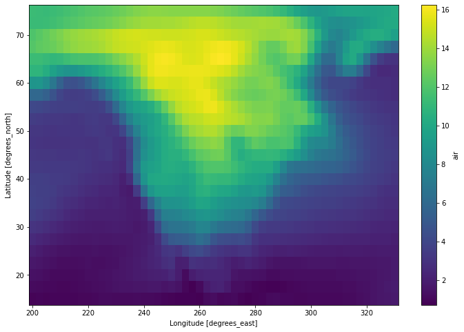
因为我们有一个 datetime 索引,时间序列操作可以高效工作。在这里我们演示 xarray 的 resample 方法的使用
[10]:
da.resample(time='1w').mean('time').std('time')
[10]:
<xarray.DataArray 'air' (lat: 25, lon: 53)>
dask.array<_sqrt, shape=(25, 53), dtype=float32, chunksize=(25, 25), chunktype=numpy.ndarray>
Coordinates:
  * lat      (lat) float32 75.0 72.5 70.0 67.5 65.0 ... 25.0 22.5 20.0 17.5 15.0
  * lon      (lon) float32 200.0 202.5 205.0 207.5 ... 322.5 325.0 327.5 330.0
[11]:
da.resample(time='1w').mean('time').std('time').load().plot(figsize=(12, 8))
[11]:
<matplotlib.collections.QuadMesh at 0x7fc71443de80>
和滑动窗口操作
[12]:
da_smooth = da.rolling(time=30).mean().persist()
da_smooth
[12]:
<xarray.DataArray 'air' (time: 2920, lat: 25, lon: 53)>
dask.array<truediv, shape=(2920, 25, 53), dtype=float64, chunksize=(2920, 25, 25), chunktype=numpy.ndarray>
Coordinates:
  * lat      (lat) float32 75.0 72.5 70.0 67.5 65.0 ... 25.0 22.5 20.0 17.5 15.0
  * lon      (lon) float32 200.0 202.5 205.0 207.5 ... 322.5 325.0 327.5 330.0
  * time     (time) datetime64[ns] 2013-01-01 ... 2014-12-31T18:00:00
Attributes:
    long_name:     4xDaily Air temperature at sigma level 995
    units:         degK
    precision:     2
    GRIB_id:       11
    GRIB_name:     TMP
    var_desc:      Air temperature
    dataset:       NMC Reanalysis
    level_desc:    Surface
    statistic:     Individual Obs
    parent_stat:   Other
actual_range: [185.16 322.1 ]由于 xarray 将其每个坐标变量存储在内存中,因此按标签进行切片非常简单且完全是延迟计算的。
[13]:
%time da.sel(time='2013-01-01T18:00:00')
CPU times: user 1.05 ms, sys: 2.82 ms, total: 3.87 ms
Wall time: 7.08 ms
[13]:
<xarray.DataArray 'air' (lat: 25, lon: 53)>
dask.array<getitem, shape=(25, 53), dtype=float32, chunksize=(25, 25), chunktype=numpy.ndarray>
Coordinates:
  * lat      (lat) float32 75.0 72.5 70.0 67.5 65.0 ... 25.0 22.5 20.0 17.5 15.0
  * lon      (lon) float32 200.0 202.5 205.0 207.5 ... 322.5 325.0 327.5 330.0
    time     datetime64[ns] 2013-01-01T18:00:00
Attributes:
    long_name:     4xDaily Air temperature at sigma level 995
    units:         degK
    precision:     2
    GRIB_id:       11
    GRIB_name:     TMP
    var_desc:      Air temperature
    dataset:       NMC Reanalysis
    level_desc:    Surface
    statistic:     Individual Obs
    parent_stat:   Other
actual_range: [185.16 322.1 ][14]:
%time da.sel(time='2013-01-01T18:00:00').load()
CPU times: user 23.5 ms, sys: 7.2 ms, total: 30.7 ms
Wall time: 91.1 ms
[14]:
<xarray.DataArray 'air' (lat: 25, lon: 53)>
array([[241.89   , 241.79999, 241.79999, ..., 234.39   , 235.5    ,
        237.59999],
       [246.29999, 245.29999, 244.2    , ..., 230.89   , 231.5    ,
        234.5    ],
       [256.6    , 254.7    , 252.09999, ..., 230.7    , 231.79999,
        236.09999],
       ...,
       [296.6    , 296.4    , 296.     , ..., 296.5    , 295.79   ,
        295.29   ],
       [297.     , 297.5    , 297.1    , ..., 296.79   , 296.6    ,
        296.29   ],
       [297.5    , 297.69998, 297.5    , ..., 297.79   , 298.     ,
        297.9    ]], dtype=float32)
Coordinates:
  * lat      (lat) float32 75.0 72.5 70.0 67.5 65.0 ... 25.0 22.5 20.0 17.5 15.0
  * lon      (lon) float32 200.0 202.5 205.0 207.5 ... 322.5 325.0 327.5 330.0
    time     datetime64[ns] 2013-01-01T18:00:00
Attributes:
    long_name:     4xDaily Air temperature at sigma level 995
    units:         degK
    precision:     2
    GRIB_id:       11
    GRIB_name:     TMP
    var_desc:      Air temperature
    dataset:       NMC Reanalysis
    level_desc:    Surface
    statistic:     Individual Obs
    parent_stat:   Other
actual_range: [185.16 322.1 ]自定义工作流程和自动并行化
几乎所有 xarray 的内置操作都适用于 Dask 数组。如果您想使用一个不是由 xarray 包装的函数,一个选项是从 xarray 对象 (.data) 中提取 Dask 数组并直接使用 Dask。
另一个选项是使用 xarray 的 apply_ufunc() 函数,它可以自动执行易于并行化的“映射”类型操作,其中为处理 NumPy 数组而编写的函数应重复应用于包含 Dask 数组的 xarray 对象。它的工作方式类似于 dask.array.map_blocks() 和 dask.array.blockwise(),但无需中间抽象层。
在这里,我们展示一个使用 NumPy 操作和 bottleneck 中的一个快速函数的示例,我们用它来计算 Spearman 秩相关系数
[15]:
import numpy as np
import xarray as xr
import bottleneck

def covariance_gufunc(x, y):
    return ((x - x.mean(axis=-1, keepdims=True))
            * (y - y.mean(axis=-1, keepdims=True))).mean(axis=-1)

def pearson_correlation_gufunc(x, y):
    return covariance_gufunc(x, y) / (x.std(axis=-1) * y.std(axis=-1))

def spearman_correlation_gufunc(x, y):
    x_ranks = bottleneck.rankdata(x, axis=-1)
    y_ranks = bottleneck.rankdata(y, axis=-1)
    return pearson_correlation_gufunc(x_ranks, y_ranks)

def spearman_correlation(x, y, dim):
    return xr.apply_ufunc(
        spearman_correlation_gufunc, x, y,
        input_core_dims=[[dim], [dim]],
        dask='parallelized',
        output_dtypes=[float])
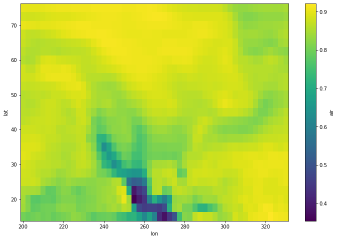
在上面的示例中,我们使用了气温数据。对于此示例,我们将使用原始气温数据与我们创建的平滑版本 (da_smooth) 来计算 spearman 相关性。为此,我们还需要提前对数据进行重新分块。
[16]:
corr = spearman_correlation(da.chunk({'time': -1}),
                            da_smooth.chunk({'time': -1}),
                            'time')
corr
[16]:
<xarray.DataArray 'air' (lat: 25, lon: 53)>
dask.array<transpose, shape=(25, 53), dtype=float64, chunksize=(25, 25), chunktype=numpy.ndarray>
Coordinates:
  * lat      (lat) float32 75.0 72.5 70.0 67.5 65.0 ... 25.0 22.5 20.0 17.5 15.0
  * lon      (lon) float32 200.0 202.5 205.0 207.5 ... 322.5 325.0 327.5 330.0
[17]:
corr.plot(figsize=(12, 8))
[17]:
<matplotlib.collections.QuadMesh at 0x7fc70cd2fdc0>