Dask 用于机器学习

Dask 用于机器学习¶

这是一个高级概述，演示了 Dask-ML 的一些组件。请访问主要的 Dask-ML 文档，参阅 dask 教程 notebook 08，或探索其他一些机器学习示例。

[1]:

from dask.distributed import Client, progress
client = Client(processes=False, threads_per_worker=4,
                n_workers=1, memory_limit='2GB')
client

[1]:

客户端

Client-12a6896d-0de0-11ed-9ba6-000d3a8f7959

连接方法： Cluster object	集群类型： distributed.LocalCluster
仪表盘： http://10.1.1.64:8787/status

集群信息

LocalCluster

ced599b8

仪表盘： http://10.1.1.64:8787/status	工作节点 1
总线程数 4	总内存： 1.86 GiB
状态：运行中	使用进程： False

调度器信息

调度器

Scheduler-60443685-4058-48d1-ba10-996f80c21c06

Comm： inproc://10.1.1.64/7078/1	工作节点 1
仪表盘： http://10.1.1.64:8787/status	总线程数 4
启动于：刚刚	总内存： 1.86 GiB

工作节点

工作节点：0

Comm： inproc://10.1.1.64/7078/4	总线程数 4
仪表盘： http://10.1.1.64:42349/status	内存： 1.86 GiB
Nanny： None
本地目录： /home/runner/work/dask-examples/dask-examples/dask-worker-space/worker-0l66zwyz

分布式训练¶

cd85db072b79444797189091746fac41

Scikit-learn 使用 joblib 实现单机并行。这允许您使用笔记本电脑或工作站的所有核心来训练大多数估计器（任何接受 n_jobs 参数的估计器）。

或者，Scikit-Learn 可以使用 Dask 实现并行。这允许您使用集群的所有核心来训练这些估计器，而无需显著更改代码。

这对于在中等大小数据集上训练大型模型最有用。当搜索大量超参数时，或者使用包含许多独立估计器的集成方法时，您可能会拥有一个大型模型。对于过小的数据集，训练时间通常很短，集群范围的并行性没有帮助。对于过大的数据集（大于单机内存），scikit-learn 估计器可能无法处理（见下文）。

创建 Scikit-Learn 估计器¶

[2]:

from sklearn.datasets import make_classification
from sklearn.svm import SVC
from sklearn.model_selection import GridSearchCV
import pandas as pd

我们将使用 scikit-learn 创建一对小的随机数组，一个用于特征 X，一个用于目标 y。

[3]:

X, y = make_classification(n_samples=1000, random_state=0)
X[:5]

[3]:

array([[-1.06377997,  0.67640868,  1.06935647, -0.21758002,  0.46021477,
        -0.39916689, -0.07918751,  1.20938491, -0.78531472, -0.17218611,
        -1.08535744, -0.99311895,  0.30693511,  0.06405769, -1.0542328 ,
        -0.52749607, -0.0741832 , -0.35562842,  1.05721416, -0.90259159],
       [ 0.0708476 , -1.69528125,  2.44944917, -0.5304942 , -0.93296221,
         2.86520354,  2.43572851, -1.61850016,  1.30071691,  0.34840246,
         0.54493439,  0.22532411,  0.60556322, -0.19210097, -0.06802699,
         0.9716812 , -1.79204799,  0.01708348, -0.37566904, -0.62323644],
       [ 0.94028404, -0.49214582,  0.67795602, -0.22775445,  1.40175261,
         1.23165333, -0.77746425,  0.01561602,  1.33171299,  1.08477266,
        -0.97805157, -0.05012039,  0.94838552, -0.17342825, -0.47767184,
         0.76089649,  1.00115812, -0.06946407,  1.35904607, -1.18958963],
       [-0.29951677,  0.75988955,  0.18280267, -1.55023271,  0.33821802,
         0.36324148, -2.10052547, -0.4380675 , -0.16639343, -0.34083531,
         0.42435643,  1.17872434,  2.8314804 ,  0.14241375, -0.20281911,
         2.40571546,  0.31330473,  0.40435568, -0.28754632, -2.8478034 ],
       [-2.63062675,  0.23103376,  0.04246253,  0.47885055,  1.54674163,
         1.6379556 , -1.53207229, -0.73444479,  0.46585484,  0.4738362 ,
         0.98981401, -1.06119392, -0.88887952,  1.23840892, -0.57282854,
        -1.27533949,  1.0030065 , -0.47712843,  0.09853558,  0.52780407]])

我们将拟合一个支持向量分类器，使用网格搜索来寻找超参数 \(C\) 的最佳值。

[4]:

param_grid = {"C": [0.001, 0.01, 0.1, 0.5, 1.0, 2.0, 5.0, 10.0],
              "kernel": ['rbf', 'poly', 'sigmoid'],
              "shrinking": [True, False]}

grid_search = GridSearchCV(SVC(gamma='auto', random_state=0, probability=True),
                           param_grid=param_grid,
                           return_train_score=False,
                           cv=3,
                           n_jobs=-1)

要正常拟合，我们会调用

grid_search.fit(X, y)

要使用集群进行拟合，我们只需要使用 joblib 提供的上下文管理器。

[5]:

import joblib

with joblib.parallel_backend('dask'):
    grid_search.fit(X, y)

我们拟合了 48 个不同的模型，对应 param_grid 中的每个超参数组合，分布在集群中。此时，我们有了一个常规的 scikit-learn 模型，可用于预测、评分等。

[6]:

pd.DataFrame(grid_search.cv_results_).head()

[6]:

	mean_fit_time	std_fit_time	mean_score_time	std_score_time	param_C	param_kernel	param_shrinking	params	split0_test_score	split1_test_score	split2_test_score	mean_test_score	std_test_score	rank_test_score
0	0.267177	0.011928	0.030591	0.006284	0.001	rbf	True	{'C': 0.001, 'kernel': 'rbf', 'shrinking': True}	0.502994	0.501502	0.501502	0.501999	0.000704	41
1	0.263738	0.005183	0.028903	0.005411	0.001	rbf	False	{'C': 0.001, 'kernel': 'rbf', 'shrinking': False}	0.502994	0.501502	0.501502	0.501999	0.000704	41
2	0.193400	0.005858	0.018773	0.003098	0.001	poly	True	{'C': 0.001, 'kernel': 'poly', 'shrinking': True}	0.502994	0.501502	0.501502	0.501999	0.000704	41
3	0.196229	0.006628	0.018826	0.002250	0.001	poly	False	{'C': 0.001, 'kernel': 'poly', 'shrinking': Fa...	0.502994	0.501502	0.501502	0.501999	0.000704	41
4	0.378106	0.006729	0.037400	0.002586	0.001	sigmoid	True	{'C': 0.001, 'kernel': 'sigmoid', 'shrinking':...	0.502994	0.501502	0.501502	0.501999	0.000704	41

[7]:

grid_search.predict(X)[:5]

[7]:

array([0, 1, 1, 1, 0])

[8]:

grid_search.score(X, y)

[8]:

0.983

有关使用分布式 joblib 训练 scikit-learn 模型的更多信息，请参阅 dask-ml 文档。

在大型数据集上训练¶

scikit-learn 中的大多数估计器都设计用于内存中的数组。使用大型数据集进行训练可能需要不同的算法。

Dask-ML 中实现的所有算法都非常适用于大于内存的数据集，您可以将其存储在 dask 数组或数据框中。

[9]:

%matplotlib inline

[10]:

import dask_ml.datasets
import dask_ml.cluster
import matplotlib.pyplot as plt

在本例中，我们将使用 dask_ml.datasets.make_blobs 生成一些随机的 dask 数组。

[11]:

X, y = dask_ml.datasets.make_blobs(n_samples=10000000,
                                   chunks=1000000,
                                   random_state=0,
                                   centers=3)
X = X.persist()
X

[11]:

	数组	块
字节	152.59 MiB	15.26 MiB
形状	(10000000, 2)	(1000000, 2)
数量	10 个任务	10 个块
类型	float64	numpy.ndarray

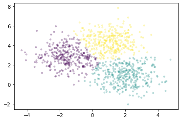
我们将使用 Dask-ML 中实现的 k-means 对点进行聚类。它使用 k-means||（读作：“k-means parallel”）初始化算法，该算法比 k-means++ 具有更好的扩展性。所有的计算，包括初始化期间和之后，都可以并行进行。

[12]:

km = dask_ml.cluster.KMeans(n_clusters=3, init_max_iter=2, oversampling_factor=10)
km.fit(X)

/usr/share/miniconda3/envs/dask-examples/lib/python3.9/site-packages/dask/base.py:1283: UserWarning: Running on a single-machine scheduler when a distributed client is active might lead to unexpected results.
  warnings.warn(

[12]:

KMeans(init_max_iter=2, n_clusters=3, oversampling_factor=10)

我们将绘制一个点样本，根据每个点所属的簇进行着色。

[13]:

fig, ax = plt.subplots()
ax.scatter(X[::10000, 0], X[::10000, 1], marker='.', c=km.labels_[::10000],
           cmap='viridis', alpha=0.25);

有关 Dask-ML 中实现的所有估计器，请参阅 API 文档。

使用 Futures 进行自定义工作负载

使用 SQL 对 Dask 数据框进行操作

Dask 示例文档