扩展 XGBoost
目录
实时 Notebook
您可以在实时会话中运行此 Notebook ![]() 或在Github 上查看。
或在Github 上查看。
扩展 XGBoost
Dask 和 XGBoost 可以协同工作,并行训练梯度提升树。本 Notebook 展示了如何一起使用 Dask 和 XGBoost。
XGBoost 提供了一个强大的预测框架,并且在实践中表现出色。它赢得了 Kaggle 竞赛,并在工业界广受欢迎,因为它具有良好的性能并且易于解释(即,很容易从 XGBoost 模型中找到重要特征)。

![]()
设置 Dask
我们设置了一个 Dask 客户端,它通过仪表盘提供性能和进度指标。
运行单元格后,点击链接即可查看仪表盘。
[1]:
from dask.distributed import Client

client = Client(n_workers=4, threads_per_worker=1)
client
[1]:
客户端
Client-ae48a4c8-0de1-11ed-a6d2-000d3a8f7959
| 连接方法: Cluster object | 集群类型: distributed.LocalCluster |
| 仪表盘: http://127.0.0.1:8787/status |
集群信息
LocalCluster
d17d0b16
| 仪表盘: http://127.0.0.1:8787/status | 工作器 4 |
| 总线程数 4 | 总内存: 6.78 GiB |
| 状态: 运行中 | 使用进程: True |
调度器信息
调度器
Scheduler-63756a1e-88c9-43fb-9a77-fb66783417d3
| 通信: tcp://127.0.0.1:36303 | 工作器 4 |
| 仪表盘: http://127.0.0.1:8787/status | 总线程数 4 |
| 启动时间: 刚刚 | 总内存: 6.78 GiB |
工作器
工作器:0
| 通信: tcp://127.0.0.1:36301 | 总线程数 1 |
| 仪表盘: http://127.0.0.1:39597/status | 内存: 1.70 GiB |
| Nanny: tcp://127.0.0.1:46201 | |
| 本地目录: /home/runner/work/dask-examples/dask-examples/machine-learning/dask-worker-space/worker-ddcw2w5v | |
工作器:1
| 通信: tcp://127.0.0.1:40821 | 总线程数 1 |
| 仪表盘: http://127.0.0.1:33095/status | 内存: 1.70 GiB |
| Nanny: tcp://127.0.0.1:36319 | |
| 本地目录: /home/runner/work/dask-examples/dask-examples/machine-learning/dask-worker-space/worker-5hsjt1n7 | |
工作器:2
| 通信: tcp://127.0.0.1:34869 | 总线程数 1 |
| 仪表盘: http://127.0.0.1:44313/status | 内存: 1.70 GiB |
| Nanny: tcp://127.0.0.1:40433 | |
| 本地目录: /home/runner/work/dask-examples/dask-examples/machine-learning/dask-worker-space/worker-a0hc6mn9 | |
工作器:3
| 通信: tcp://127.0.0.1:44521 | 总线程数 1 |
| 仪表盘: http://127.0.0.1:38003/status | 内存: 1.70 GiB |
| Nanny: tcp://127.0.0.1:34813 | |
| 本地目录: /home/runner/work/dask-examples/dask-examples/machine-learning/dask-worker-space/worker-r6mejztr | |
创建数据
首先,我们创建大量合成数据,包含 100,000 个样本和 20 个特征。
[2]:
from dask_ml.datasets import make_classification

X, y = make_classification(n_samples=100000, n_features=20,
                           chunks=1000, n_informative=4,
                           random_state=0)
X
/usr/share/miniconda3/envs/dask-examples/lib/python3.9/site-packages/dask/base.py:1283: UserWarning: Running on a single-machine scheduler when a distributed client is active might lead to unexpected results.
  warnings.warn(
[2]:
|
Dask-XGBoost 支持数组和 DataFrames。有关从真实数据创建 Dask 数组和 DataFrames 的更多信息,请参阅 Dask 数组或Dask dataframes 的文档。
拆分训练和测试数据
我们将数据集拆分为训练和测试数据,以确保进行公平的测试,从而辅助评估。
[3]:
from dask_ml.model_selection import train_test_split

X_train, X_test, y_train, y_test = train_test_split(X, y, test_size=0.15)
现在,我们尝试使用 dask-xgboost 对这些数据进行处理。
训练 Dask-XGBoost
[4]:
import dask
import xgboost
import dask_xgboost
/usr/share/miniconda3/envs/dask-examples/lib/python3.9/site-packages/xgboost/compat.py:36: FutureWarning: pandas.Int64Index is deprecated and will be removed from pandas in a future version. Use pandas.Index with the appropriate dtype instead.
  from pandas import MultiIndex, Int64Index
dask-xgboost 是 xgboost 的一个小型包装器。Dask 设置 XGBoost,提供数据给 XGBoost,并让 XGBoost 在后台利用 Dask 可用的所有工作器进行训练。
让我们进行训练
[5]:
params = {'objective': 'binary:logistic',
          'max_depth': 4, 'eta': 0.01, 'subsample': 0.5,
          'min_child_weight': 0.5}

bst = dask_xgboost.train(client, params, X_train, y_train, num_boost_round=10)
Exception in thread Thread-4:
Traceback (most recent call last):
  File "/usr/share/miniconda3/envs/dask-examples/lib/python3.9/threading.py", line 973, in _bootstrap_inner
    self.run()
  File "/usr/share/miniconda3/envs/dask-examples/lib/python3.9/threading.py", line 910, in run
    self._target(*self._args, **self._kwargs)
  File "/usr/share/miniconda3/envs/dask-examples/lib/python3.9/site-packages/dask_xgboost/tracker.py", line 365, in join
    while self.thread.isAlive():
AttributeError: 'Thread' object has no attribute 'isAlive'
可视化结果
该 bst 对象是一个常规的 xgboost.Booster 对象。
[6]:
bst
[6]:
<xgboost.core.Booster at 0x7ff9c8b16610>
这意味着XGBoost 文档中提到的所有方法都可用。我们展示两个例子来详细说明,但这些例子是关于 XGBoost 而不是 Dask 的。
绘制特征重要性
[7]:
%matplotlib inline
import matplotlib.pyplot as plt

ax = xgboost.plot_importance(bst, height=0.8, max_num_features=9)
ax.grid(False, axis="y")
ax.set_title('Estimated feature importance')
plt.show()
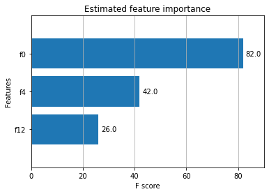
我们创建数据时指定只有 4 个特征具有信息量,而只有 3 个特征显示为重要。
绘制接收者操作特征曲线
我们可以使用一个更高级的指标来确定分类器的性能,即绘制接收者操作特征 (ROC) 曲线。
[8]:
y_hat = dask_xgboost.predict(client, bst, X_test).persist()
y_hat
[19:24:16] WARNING: /home/conda/feedstock_root/build_artifacts/xgboost-split_1645117766796/work/src/learner.cc:1264: Empty dataset at worker: 0
[8]:
|
[9]:
from sklearn.metrics import roc_curve

y_test, y_hat = dask.compute(y_test, y_hat)
fpr, tpr, _ = roc_curve(y_test, y_hat)
[10]:
from sklearn.metrics import auc

fig, ax = plt.subplots(figsize=(5, 5))
ax.plot(fpr, tpr, lw=3,
        label='ROC Curve (area = {:.2f})'.format(auc(fpr, tpr)))
ax.plot([0, 1], [0, 1], 'k--', lw=2)
ax.set(
    xlim=(0, 1),
    ylim=(0, 1),
    title="ROC Curve",
    xlabel="False Positive Rate",
    ylabel="True Positive Rate",
)
ax.legend();
plt.show()
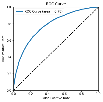
这条接收者操作特征 (ROC) 曲线显示了我们的分类器性能如何。通过观察它向左上方弯曲的程度,我们可以判断它的性能。一个完美的分类器会位于左上方角落,而一个随机分类器会沿着对角线。
这条曲线下的面积是 area = 0.76。这告诉我们分类器对于随机选择的实例进行正确预测的概率。
了解更多
录制的截屏视频,逐步演示上面的真实世界示例
关于 dask-xgboost 的博文 http://matthewrocklin.com/blog/work/2017/03/28/dask-xgboost
XGBoost 文档:https://docs.xgboost.com.cn/en/latest/python/python_intro.html#
Dask-XGBoost 文档:https://ml.dask.org.cn/xgboost.html